statistics
Statistics
If a variant X takes values x1, x2, x3…. xn with corresponding frequencies f1, f2, f3 ,… fn respectively, then arithmetic mean of these values is given by:
−X=∑ni=1fixiN where N=n∑i=1f1+f2+f2……..+fn
Let x1, x2….,xn be values of a variable X with corresponding frequencies f1, f2, f3 ,fn respectively. Let A be the assumed mean. Then:
−X=A+1N{n∑i=1fidi}
Note that in case of continuous frequency distribution, the values of x1, x2, x3 … xn, are taken as the mid-points or class-marks of the various classes.
Let x1, x2….,xn be values of a variable X with corresponding frequencies f1, f2, f3 ,…..fn respectively. Let A be the assumed mean. Then:
−X=A+h{1Nn∑i=1fiui}
Here, h is generally taken as common factor of the deviations, in case of ungrouped frequency distribution. And, in case of grouped frequency distribution, h is the class width, ui=xi−Ah=dih
Note that in case of continuous frequency distribution, the values of x1, x2, x3 …, xn are taken as the mid-points or class-marks of the various classes.
If n is even, then median is the arithmetic mean of the values of (n2)thand (n2+1)th observations.
Step 1: Find the cumulative frequencies (c.f.) and obtain N =∑f1.
Step 2: Find n2
Step 3: Look for the cumulative frequency (c. f.) just greater than n2 and determine the corresponding value of the variable. The value so obtained is the median.
Step 1: Find the cumulative frequencies (c.f.) and obtain N =∑f1.
Step 2: Find N2
Step 3: Look for the cumulative frequency (c. f.) just greater than N2 and determine the correspondingclass. This class is known as the median class. (Note that the value of the median will lie in this class)
Step 4: Use the following formula to find median:
Mediun=l+⎡⎣N2−cff⎤⎦×h
Here, l = lower limit of the median class
f = frequency of the median class
h = width (size) of the median class
cf = cumulative frequency of the class preceding the median class
N =∑f1 .
mode can be calculated by the following formula
Mode=l+f1−f02f1−f0−f2×h
l = lower limit of the modal class
h = size of the class interval
f1 = frequency of the modal class
f0 =frequency of the class preceding the modal class
f2 = frequency of the class succeeding the modal class
Negatively skewed distributions have a few extremely low scores, while positively skewed distributions have a few extremely high scores.
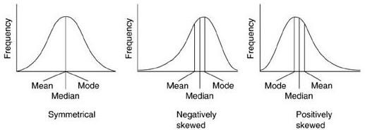 When the positively skewed, then Mean > Median > Mode
Three measure of central values are connected by the following relation:
3 Median = Mode + 2 Mean
Step 1: Draw more than or less than ogive as asked in question. Find of observations.N2 where N is the total number
Step 2: Locate the N2 cumulative frequency on the y-axis.
Step 3: Draw a line parallel to x-axis through the point obtained in step 2, cutting the cumulative frequency curve at a point P (say).
Step 4: Draw perpendicular PM from P on the x-axis. The x-coordinate of point M is the median value.
Step 1: Draw both ogives on the same graph.
Step 2: Identify the point of intersection of both ogives and mark it as Q (say).
Step 3: Draw perpendicular from Q on x-axis.
Step 4: The point of perpendicular on x-axis is the median.
Ungrouped Data
Ungrouped data is data in its original or raw form. The observations are not classified into groups.
For example, the ages of everyone present in a classroom of kindergarten kids with the teacher is as follows:
3, 3, 4, 3, 5, 4, 3, 3, 4, 3, 3, 3, 3, 4, 3, 27.
This data shows that there is one adult present in this class and that is the teacher. Ungrouped data is easy to work with when the data set is small.
Grouped Data
In grouped data, observations are organized in groups.
For example, a class of students got different marks in a school exam. The data is tabulated as follows:
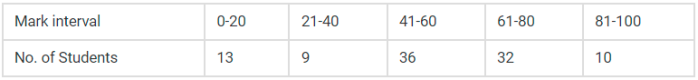
This shows how many students got the particular mark range. Grouped data is easier to work with when a large amount of data is present.
Frequency
Frequency is the number of times a particular observation occurs in data.
Class Interval
Data can be grouped into class intervals such that all observations in that range belong to that class.
Class width = upper class limit – lower class limit
Mean
Finding the mean for Grouped Data when class Intervals are not given
For grouped data without class intervals,
Mean = ¯¯¯x=∑xifi∑fi
where fi is the frequency of ith observation xi.
Finding the mean for Grouped Data when class Intervals are given
For grouped data with class intervals,
Mean = ¯¯¯x=∑xifi∑fi
Where fi is the frequency of ith class whose class mark is xi.
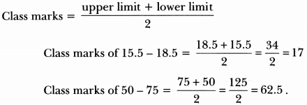
Classmark = (Upper Class Limit+ Lower Class Limit)/2
Direct method of finding mean
Step 1: Classify the data into intervals and find the corresponding frequency of each class.
Step 2: Find the class mark by taking the midpoint of the upper and lower class limits.
Step 3: Tabulate the product of the class mark and its corresponding frequency for each class. Calculate their sum (∑xifi).
Step 4: Divide the above sum by the sum of frequencies (∑fi) to get the mean.
Assumed mean method of finding mean
Step 1: Classify the data into intervals and find the corresponding frequency of each class.
Step 2: Find the class mark by taking the midpoint of the upper and lower class limits.
Step 3: Take one of the xi’s (usually one in the middle) as the assumed mean and denote it by ′a′.
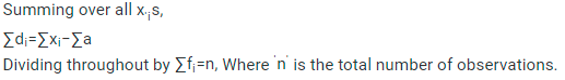
Step 4: Find the deviation of ′a′ from each of the x′is
di = xi − a
Step 5: Find the mean of the deviations
¯¯¯d=∑fidi∑fi
Step 6: Calculate the mean as
¯¯¯x=a+∑fidi∑fi
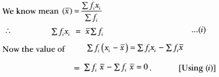
The relation between the Mean of deviations and mean
![]()
![]()
Step-Deviation method of finding mean
Step 1: Classify the data into intervals and find the corresponding frequency of each class.
Step 2: Find the class mark by taking the midpoint of the upper and lower class limits.
Step 3: Take one of the x′is (usually one in the middle) as assumed mean and denote it by ′a′.
Step 4: Find the deviation of a from each of the x′is
di = xi − a
Step 5: Divide all deviations −di by the class width (h) to get u′is.
ui=xi−ah
Step 6: Find the mean of u′is
¯¯¯u=∑fiui∑fi
Step 7: Calculate the mean as
¯¯¯x=a+h×∑fiui∑fi=a+h¯¯¯u
Relation between mean of Step- Deviations (u) and mean
ui=xi−ah
¯¯¯u=∑fixi−ah∑fi
¯¯¯u=1h×∑fixi−a∑fi∑fi
¯¯¯u=1h×(¯¯¯x−a)
Important relations between methods of finding mean
Median
Finding the Median of Grouped Data when class Intervals are not given
Step 1: Tabulate the observations and the corresponding frequency in ascending or descending order.
Step 2: Add the cumulative frequency column to the table by finding the cumulative frequency up to each observation.
Step 3: If the number of observations is odd, the median is the observation whose cumulative frequency is just greater than or equal to (n+1)/2
If the number of observations is even, the median is the average of observations whose cumulative frequency is just greater than or equal to n/2 and (n/2)+1.
Cumulative Frequency
Cumulative frequency is obtained by adding all the frequencies up to a certain point.
Finding median for Grouped Data when class Intervals are given
Step 1: find the cumulative frequency for all class intervals.
Step 2: the median class is the class whose cumulative frequency is greater than or nearest to n2, where n is the number of observations.
Step 3: Median = l + [(N/2 – cf)/f] × h
Where,
l = lower limit of median class,
n = number of observations,
cf = cumulative frequency of class preceding the median class,
f = frequency of median class,
h = class size (assuming class size to be equal).
Cumulative Frequency distribution of less than type
Cumulative frequency of the less than type indicates the number of observations which are less than or equal to a particular observation.
Cumulative Frequency distribution of more than type
Cumulative frequency of more than type indicates the number of observations that are greater than or equal to a particular observation.
Visualising formula for median graphically
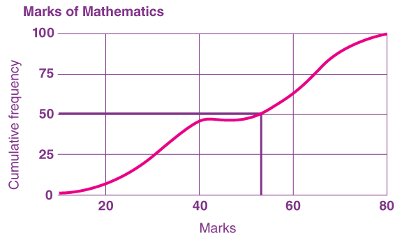
Median from Cumulative Frequency Curve
Step 1: Identify the median class.
Step 2: Mark cumulative frequencies on the y-axis and observations on the x-axis corresponding to the median class.
Step 3: Draw a straight line graph joining the extremes of class and cumulative frequencies.
Step 4: Identify the point on the graph corresponding to cf = n/2
Step 5: Drop a perpendicular from this point onto the x-axis.
Ogive of less than type
The graph of a cumulative frequency distribution of the less than type is called an ‘ogive of the less than type’.
Ogive of more than type
The graph of a cumulative frequency distribution of the more than type is called an ‘ogive of the more than type’.
Relation between the less than and more than type curves
The point of intersection of the ogives of more than and less than types gives the median of the grouped frequency distribution.
Mode
Finding mode for Grouped Data when class intervals are not given
In grouped data without class intervals, the observation having the largest frequency is the mode.
Finding mode for Ungrouped Data
For ungrouped data, the mode can be found out by counting the observations and using tally marks to construct a frequency table.
The observation having the largest frequency is the mode.
Important Questions
Multiple Choice questions-
1. Cumulative frequency curve is also called
(a) histogram
(b) ogive
(c) bar graph
(d) median
2. The relationship between mean, median and mode for a moderately skewed distribution is
(a) mode = median – 2 mean
(b) mode = 3 median – 2 mean
(c) mode = 2 median – 3 mean
(d) mode = median – mean
3. The median of set of 9 distinct observations is 20.5. If each of the largest 4 observations of the set is increased by 2, then the median of the new set
(a) is increased by 2
(b) is decreased by 2
(c) is two times of the original number
(d) Remains the same as that of the original set.
4. Mode and mean of a data are 12k and 15A. Median of the data is
(a) 12k
(b) 14k
(c) 15k
(d) 16k
5. The times, in seconds, taken by 150 atheletes to run a 110 m hurdle race are tabulated below:
|
Class |
Frequency |
|
13.8 – 14.0 |
2 |
|
14.0 – 14.2 |
4 |
|
14.2 – 14.4 |
5 |
|
14.4 – 14.6 |
71 |
|
14.6 – 14.8 |
48 |
|
14.8 – 15.0 |
20 |
The number of atheletes who completed the race in less then 14.6 seconds is:
(a) 11
(b) 71
(c) 82
(d) 130
6. The abscissa of the point of intersection of the less than type and of the more than type cumulative frequency curves of a grouped data gives its
(a) mean
(b) median
(c) mode
(d) all the three above
7. While computing mean of grouped data, we assume that the frequencies are:
(a) evenly distributed over all the classes
(b) centred at the classmarks of the classes
(c) centred at the upper limits of the classes
(d) centred at the lower limits of the classes
8. Mean of 100 items is 49. It was discovered that three items which should have been 60, 70, 80 were wrongly read as 40, 20, 50 respectively. The correct mean is
(a) 48
(b) 49
(c) 50
(d) 60
9. While computing mean of grouped data, we assume that the frequencies are
(a) centred at the upper limits of the classes
(b) centred at the lower limits of the classes
(c) centred at the classmarks of the classes
(d) evenly distributed over all the classes
10. Which of the following can not be determined graphically?
(a) Mean
(b) Median
(c) Mode
(d) None of these
Very Short Questions:
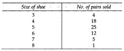
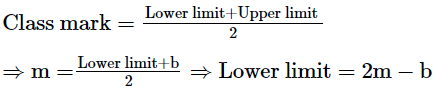
Find the model size of the shoes sold.
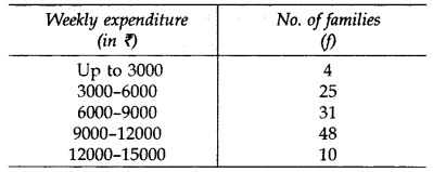
Find the upper limit of the modal class.
Short Questions :

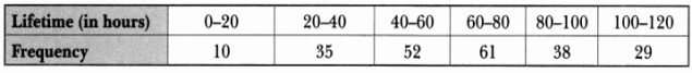
Determine the modal lifetimes of the components.
Long Questions :

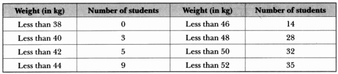
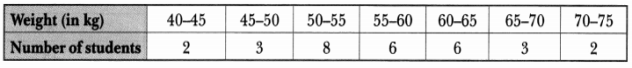
Draw a less than type ogive for the given data. Hence, obtain the median weight from the graph and verify the result by using the formula.
Case Study Questions:


Assertion Reason Questions-
Assertion: median= ((n+1)/2)th value if n is odd
Reason: If the number of runs scored by 11 players of a cricket team of India are 5, 19, 42, 11, 50, 30, 21, 0, 52, 36, 27 then median is 30
Assertion: if the value of mode and mean is 60 and 66 then the value of median is 64.
Reason: median = (mode + 2mean)
Answer Key-
Multiple Choice questions-
Very Short Answer :
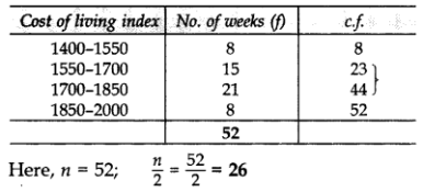
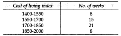
∴ Median class 1700 – 1850.
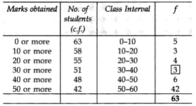
∴ Frequency of class 30 – 40 = 3
∴ Modal size of shoes = 5
∴ Modal class = 9,000 – 12,000
Upper limit of the modal class = 12,000
![]()
![]()
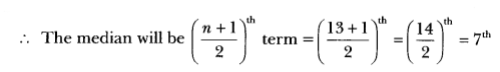
i.e., 7th term will be the median.
Relation among mean, median and mode is
3 median = mode + 2 mean
3 × median = 8 + 2 × 8
Median = 8+163 = 243 = 8
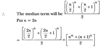
i.e., the mean of nth and (n + 1)th term will be the median.
Short Answer :
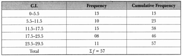
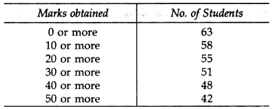
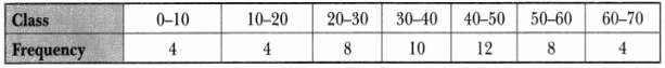
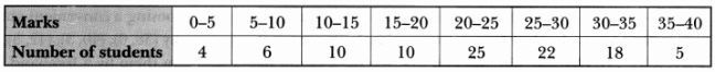
Class interval can’t be negative hence the first CI is starting from 0.
Now to find median class we calculate Σf2=572= 28.5
∴ Median class = 11.5 – 17.5.
So, the upper limit is 17.5
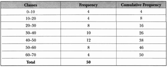
Here, n2 = 502
∴ Median class = 30 – 40.
So, the modal class is 60 – 80.
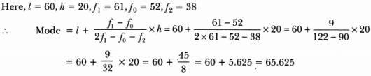
Hence, modal lifetime of the components is 65.625 hours.
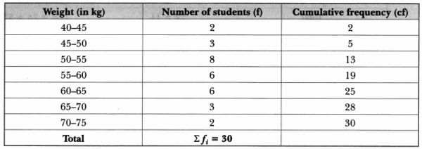
The cumulative frequency just greater than n2 = 15 is 19, and the corresponding class is 55 – 60.
∴ 55 – 60 is the median class.
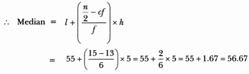
Hence, median weight is 56.67 kg.
Long Answer :
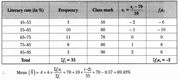
Let assumed mean A = 70 and class size h = 10
So, ui = xi−7010
Now, we have
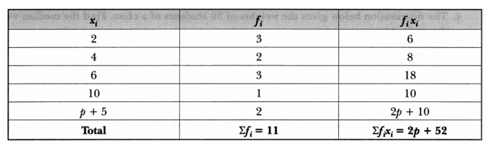
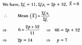
Now, we have,
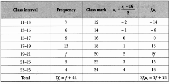
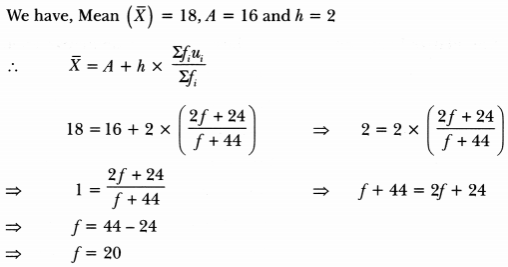
Hence, the missing frequency is 20.
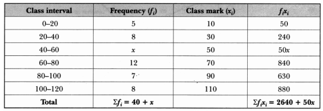
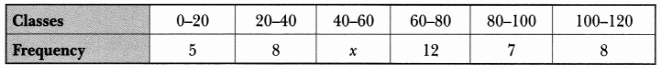
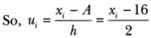
![]()
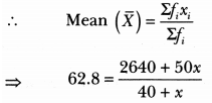
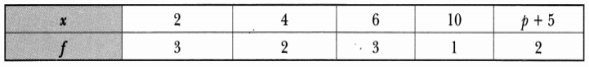
⇒ 2512 + 62.8x = 2640 + 50x
⇒ 62.8x – 50x = 2640 – 2512
⇒ 12.8x = 128
∴ x =12812.8 = 10
Hence, the missing frequency is 10.
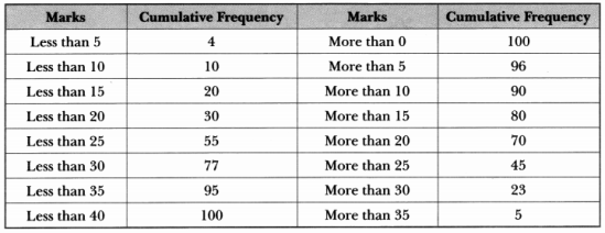
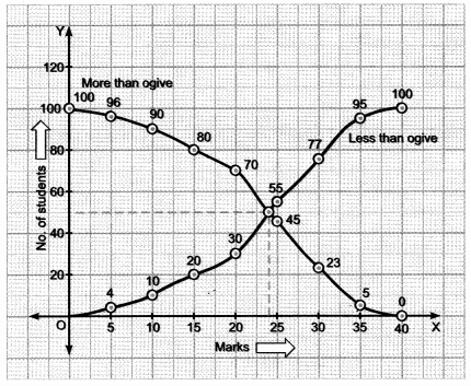
Hence, median marks = 24
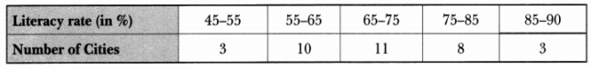
Thus, the curve obtained is the less than type ogive.
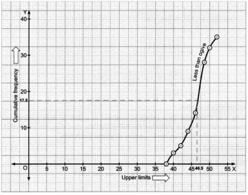
Now, locate n2=352= 17.5 on the y-axis,
We draw a line from this point parallel to x-axis cutting the curve at a point. From this point, draw a perpendicular line to the x-axis. The point of intersection of this perpendicular with the x-axis gives the median of the data. Here it is 46.5.
Let us make the following table in order to find median by using formula.
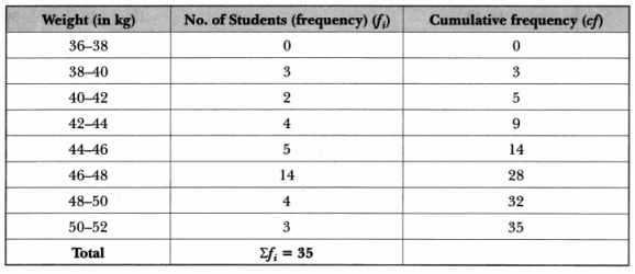
Here, n = 35, n2 = 352 = 17.5, cumulative frequency greater than n2 = 17.5 is 28 and corresponding class is 46 – 48. So median class is 46 – 48.
Now, we have l = 46, n2 = 17.5, cf = 14, f = 14, h = 2
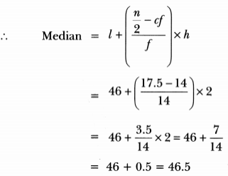
Hence, median is verified.
Case Study Answer-
Solution:
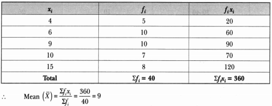
If fi and xi are very small, then direct method is appropriate method for calculating mean.
Solution:
The frequency distribution table from the given data can be drawn as:

Solution:
If 2000 vehicles comes daily and average quantity of diesel required for a vehicle is 8.15 liters, then total quantity of diesel required,
= 2000 × 8.15 = 16300 liters
Solution:
![]()
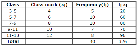
c.f. for the distribution are 5, 15, 25, 32, 40
Now, cf just greater than 20 is 25 which is corresponding to the class interval 7 – 9.
So median class is 7 – 9.
∴ Required sum of upper limit and lower limit = 7 + 9 = 16
Solution:
We know, Mode = 3 Median – 2 Mean
= 3(8) – 2(8.15) = 24 – 16.3 = 7.7
Solution:
We know that,
Solution:
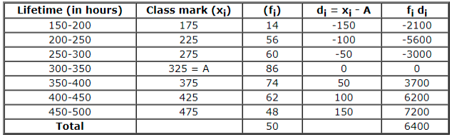
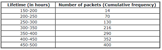
∴ Average lifetime of a packet
![]()
Solution:
![]()
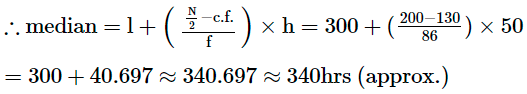
Also, cumulative frequency for the given distribution are 14, 70, 130, 216, 290, 352, 400
∴ c.f just greater than 200 is 216, which is corresponding to the interval 300-350.
l = 300, f = 86, c.f. = 130, h = 50
Solution:
We know that Mode = 3 Median – 2 Mean
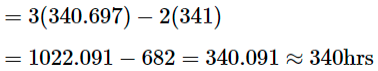
Solution:
Since, minimum of mean, median and mode is approximately 340hrs. So, manufacturer should claim that lifetime of a packet is 340hrs.
Assertion Reason Answer-
(c) A is true but R is false.
(c) A is true but R is false.